Introduction
Response surface methodology (RSM) refers to a set of statistical methods for the design of experiments, modeling of responses, and optimization of factor levels (Myers et al., 2009). RSM has extensively been used in experimental sciences, including the food science of animal resources. In RSM, a satisfactory modeling of responses is crucial for an accurate understanding of the response system and a precise optimization of explanatory factors. A model can be said to be satisfactory when: (1) the model is significant at the 5% level (the p-value of the model≤0.05), (2) the lack of fit is non-significant at the 5% level (the p-value of the lack of fit>0.05) or the model has no lack of fit, and (3) the adjusted r-square is as large as at least 0.8 (≥0.8).
In RSM, after obtaining data from an experiment, we fit a standard second-order model to the data and then check whether the above three criteria are met. If not all three criteria are met, the second-order model is unsatisfactory. Subsequently, we fit a “balanced higher-order model” to the data and check whether the above three criteria are met. If still not all three criteria are met, the balanced higher-order model too is unsatisfactory, and we fit a “balanced highest-order model” to the data. This three-step sequential modeling can be summarized as follows:
-
Step 1: Fit a second-order model to the data. If this model is satisfactory, modeling stops here. Otherwise, go to step 2.
-
Step 2: Fit a balanced higher-order model to the data. If this model is satisfactory, modeling stops here. Otherwise, go to step 3.
-
Step 3: Fit a balanced highest-order model to the data.
When each factor of the experimental design has five levels, a balanced higher-order model in step 2 is a third-order model, and a balanced highest-order model in step 3 is the fullest balanced model proposed by Rheem et al. (2017). These models used in Rheem et al. (2017) contain cubic terms in the form of Xj3. When each factor of the design has three levels that are coded as –1, 0, and 1, these models cannot be used, as cubic terms cannot be entered into the model because they are the same as linear terms [(–1)3=–1, 03=0, and 13=1, that is, Xj3=Xj)]. Thus, when each factor has three levels, the balanced higher-order and balanced highest-order models that have no cubic terms in them are required. The construction of such models will be explained later.
The present study proposes a three-step modeling strategy for experiments where each factor of the design has three levels, and subsequently optimizes factor levels for maximizing the response based on the balanced highest-order model. The study was conducted using the data from a three-level, two-factor experiment on a coffee-supplemented milk beverage (Ahn et al., 2017; Rheem et al., 2019).
Materials and Methods
The construction of a balanced highest-order model will be explained through re-analysis of a dataset from the experimental data in the article titled “Improving the Quality of Response Surface Analysis of an Experiment for Coffee-supplemented Milk Beverage: II. Heterogeneous Third-order Models and Multi-response Optimization” authored by Rheem et al. (2019). In that study, two three-level factors were used in an experiment. Among the responses in that experiment, the Zeta-potential, for which the objective of optimization is maximization, is the Y variable in this study. To illustrate the model for the data from a three-level, two-factor design, the factors (the X1 and X2 variables) in this experiment and their coded and actual levels are presented in Table 1.
The dataset used for re-analysis was the data in Rheem et al. (2019) from which the first center run was deleted. The data in Rheem et al. (2019) was obtained through the screening (Rheem and Oh, 2019) of the original data in Ahn et al. (2017). The dataset that was analyzed in this study is presented in Table 2. In this dataset, the experimental design is the central composite design by Box and Wilson (1951) for two factors having –1, 0, and 1 as their coded levels. With this dataset, we performed a response surface analysis using balanced higher-order and balanced highest-order models.
| Standard order | Design point | X1 | X2 | Y |
|---|---|---|---|---|
| 1 | 1 | –1 | –1 | 27.5 |
| 2 | 2 | –1 | 1 | 29.9667 |
| 3 | 3 | 1 | –1 | 24.3 |
| 4 | 4 | 1 | 1 | 32.5666 |
| 5 | 5 | –1 | 0 | 36.1 |
| 6 | 6 | 1 | 0 | 28.2667 |
| 7 | 7 | 0 | –1 | 29.1 |
| 8 | 8 | 0 | 1 | 28.2 |
| 9 | 9 | 0 | 0 | 29.0667 |
| 10 | 9 | 0 | 0 | 29.6 |
| 11 | 9 | 0 | 0 | 29.1 |
Data were analyzed using the SAS software. SAS (2016b) procedures were used for the modeling of the response and the drawing of a contour plot. The optimization of factor levels was performed by SAS data-step programming. A three-dimensional plot was generated using SAS (2016a).
Results and Discussion
First, the second-order polynomial regression model containing two linear, two quadratic, and one interaction term was fitted to the data by using the RSREG procedure of SAS/STAT. Results of the analysis of variance for the second-order model are shown in Table 3.
| Test of lack of fit | |||||
|---|---|---|---|---|---|
| Source | Degrees of freedom | Sum of squares | Mean square | F-value | p-value |
| Lack of fit | 3 | 37.67 | 12.56 | 140.69 | 0.0071 |
| Pure error | 2 | 0.18 | 0.09 | ||
Table 3 says that: (1) the model is non-significant at the 5% level (the p-value of the model=0.3338>0.05), (2) the lack of fit is significant at the 5% level (the p-value of the lack of fit=0.0071<0.05), and (3) the adjusted r-square=0.1388<0.8; none of the three criteria were satisfied, and thus, this model was unsatisfactory. As the second-order model had a poor fit, we proceeded to build a balanced higher-order model.
In a multifactor polynomial regression model, if each factor appears the same number of times in all the terms in the model, such a model is said to be “balanced.” In a balanced response surface model, each factor has an equal opportunity of being evaluated through the coefficients of the model terms that contain it.
When there are two factors, a second-order model, which consists of X1, X2; X12, X22; and X1X2, is balanced, because for j=1 and 2, each Xj appears three times in all the terms (1 time in X1, X2; 2 times in X12, X22; and 1 time in X1X2) in the model. Thus, the balanced higher-order model consists of X1, X2; X12, X22; X1X2; X1X22, X12X2, where for j=1 and 2, each Xj appears 7 times (1 time in X1, X2, 2 times in X12, X22, and 1 time in X1X2, and 3 times in X1X22, X12X2). Table 4 shows the results of the analysis of variance for the balanced higher-order model.
| Test of lack of fit | |||||
|---|---|---|---|---|---|
| Source | Degrees of freedom | Sum of squares | Mean square | F-value | p-value |
| Lack of fit | 1 | 5.66 | 5.66 | 63.45 | 0.0154 |
| Pure error | 2 | 0.18 | 0.09 | ||
Table 4 says that: (1) the model is non-significant at the 5% level (the p-value of the model=0.0841>0.05), (2) the lack of fit is significant at the 5% level (the p-value of the lack of fit=0.0154<0.05), and (3) the adjusted r-square=0.7785<0.8; none of the three criteria were satisfied, and thus, the balanced higher-order model was also unsatisfactory. Therefore, for the next step of model fitting, a balanced highest-order model was fitted to the data.
In Table 4, the lack of fit had one degree of freedom, implying that we can add one more term to the model. For the model to be balanced, this additional term needs to contain all of X1 and X2. As the last terms in the model are X1X22 and X12X2, the next term to be entered into the model should be X12X22. When we add this term to the model, the model becomes a balanced highest-order model, which has no lack of fit, because the number of coefficients in the model is the same as the number of design points in the experimental design. Design points are indicated in Table 2. Results of the analysis of variance for the balanced highest-order model are presented in Table 5.
| Test of lack of fit | |||||
|---|---|---|---|---|---|
| Source | Degrees of freedom | Sum of squares | Mean square | F-value | p-value |
| Lack of fit | 0 | 0 | |||
| Pure error | 2 | 0.18 | 0.09 | ||
Table 5 says that: (1) the model is significant at the 5% level (the p-value of the model=0.0081<0.05), (2) the model has no lack of fit, and (3) the adjusted r-square=0.9898>0.8; all three criteria were satisfied, and the r-square was 0.9980, almost equal to 1. Therefore, the balanced highest-order model was satisfactory and accepted as our final model. With Ŷ denoting the predicted value of Y, this model can be specified as:
Table 6 shows the coefficient estimates and their SEs, t-values, and p-values of the balanced higher-order model.
The p-values in Table 6 say that the X1, X12, X1X2, X1X22, X12X2, and X12X22 terms, which all involve the X1 factor, are all significant at the 5% level, whereas the X2 and X22 terms, which involve only the X2 factor, are non-significant at the 5% level. From this, we see that the X1 factor plays a more important role than the X2 factor in the model.
According to Ahn et al. (2017), the objective of optimization for Y was maximization. Thus, using a search on a grid (Oh et al., 1995), we optimized the model for maximization in the form of the above equation. In this experiment, the bounds were –1≤Xj≤1 for j=1, 2. Thus, within these bounds, we conducted a search on a grid using the SAS data step programming. A search for the maximum on a grid was performed by calculating the Ŷ function over a grid for the values of X1 and X2, with an increment of 0.01 within the bounds –1≤Xj≤1 for j=1, 2, and then sorting the calculated function values in descending order. The optimum point at which Ŷ was maximized was found this way and is presented in Table 7.
| X1 | X2 | F1=Speed of primary homogenization (rpm) | F2=Concentration of emulsifier (%) | Predicted maximum of Y (=Zeta-potential) |
|---|---|---|---|---|
| −1 | 0.08 | 5,000 | 0.208 | 36.1515 |
In Rheem et el. (2019), the predicted maximum Zeta-potential based on their model was 35.2957, which is lower than 36.1515, our predicted maximum Zeta-potential in Table 7. And, according to the data and the model in Rheem et el. (2019), for their predicted maximum (35.2957) of Zeta-potential, their predicted optimum points of (X1, X2) in coded levels and (F1, F2) in actual levels are calculated as (X1=–1, X2=0.10) and (F1=5.000, F1=0.210), which are different from (X1=–1, X2=0.08) and (F1=5.000, F1=0.208), our predicted optimum points in coded and actual levels in Table 7. Thus, it can be said that our approach has predicted improved results of optimization, which are different from the predicted optimization results in the previous research. A validation experiment is needed after the optimum point is predicted.
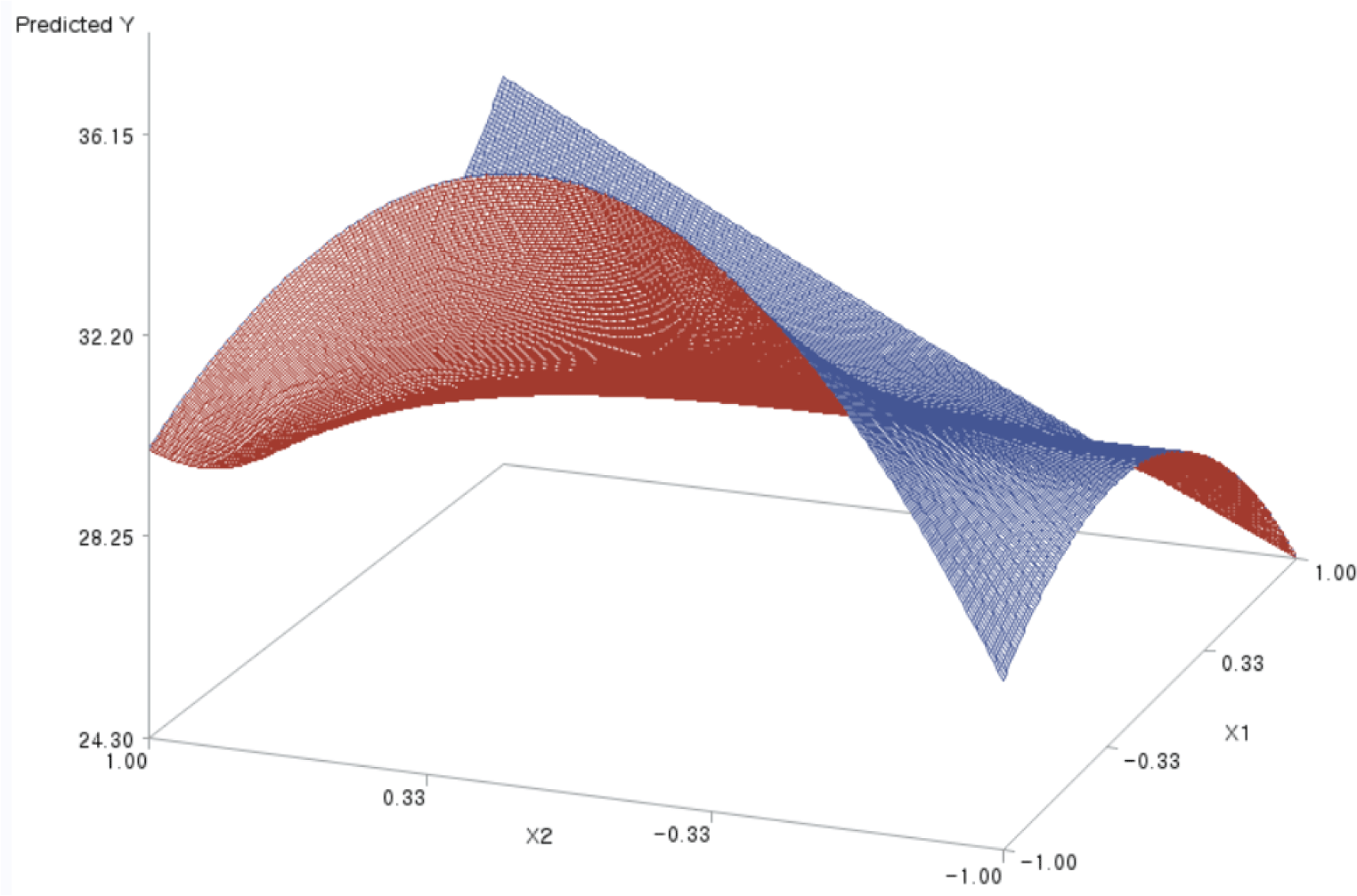
For the X1 and X2 factors, the three-dimensional (3D) response surface plot was drawn, with the vertical axis representing the predicted response and two horizontal axes indicating the coded levels of the X1 and X2 factors. Fig. 1 is such a plot.
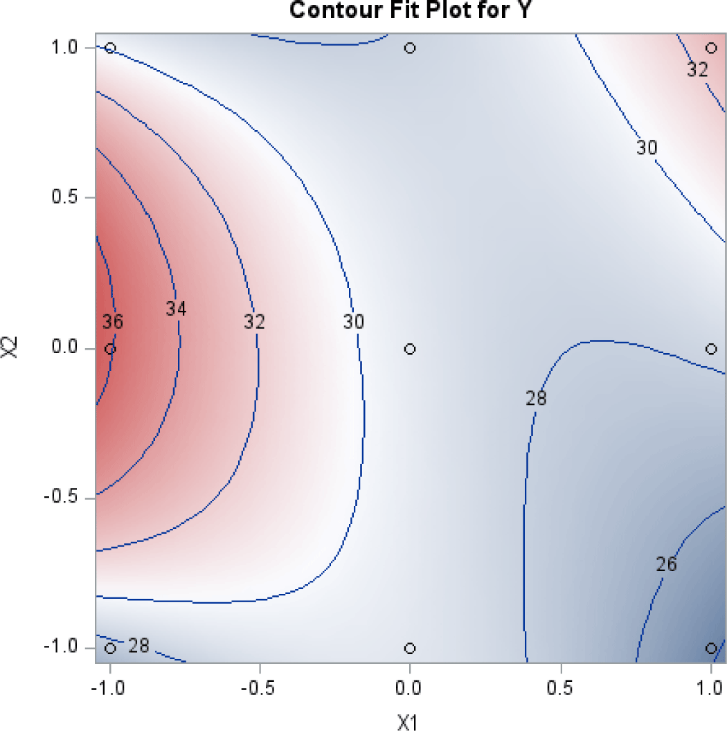
The two-dimensional contour plot of the response surface was also drawn, with two axes indicating two coded factors. Fig. 2 is such a plot.
These figures visualize the optimization results shown in Table 7; they show that the predicted response was maximized at the point of (X1=–1, X2=0.08).


