Introduction
In food science of animal resources, for the design and analysis of experiments, response surface methodology (RSM) is frequently used. RSM is a collection of statistical methods to design experiments, model data, and optimize responses (Myers et al., 2009). Among experimental plans in RSM, central composite designs (CCD, Box and Wilson, 1951) are most popular.
A CCD consists of the three portions that are factorial runs, axial runs, and center runs. Among these portions, center runs, which are the experimental runs at the center point, give some desirable properties to the design, and allow us to measure the amount of variation in the responses at the center point, providing a basis for the lack-of-fit test.
Thus, at the center point, a reasonable amount of variation in the responses is anticipated, which is measured as the pure error variance. This means that there should be no outliers among the responses at the center runs. If outliers, which are the observations extremely different from others, exist at the center point, it may imply that, at the runs that have produced outliers, there have occurred failures in keeping the experimental conditions homogeneous.
The bad influence of an outlier at the center point on statistical modeling is enormous! It is much worse than researchers think. It simply ruins statistical modeling, which views a response as the function plus a variation. An outlier at the center point is seriously detrimental to both estimating the function and measuring the amount of variation. If statistical modeling were cooking and raw data were ingredients, outliers at the center point would be a poisonous, toxic ingredient. They must be either corrected or eliminated. Even one outlier can ruin the statistical analysis of the data that were obtained through a research into which a lot of expenses and manpower is invested. It is possible that just one outlier makes the result of a highly cost research unreliable.
A remedy for the situation where outliers are observed at the center point is simple. It is either the correction or the elimination of such outliers. Therefore, we suggest the following: “Before fitting a statistical model, look at the responses at the center point. If the outliers are observed at the center point, examine them. If they are due to errors in measuring or typing, correct them, otherwise, delete them.” This is what we mean by data screening at the center point.
This research was motivated by our seeing a situation where a serious outlier at the center point exists and it is overlooked, and, accordingly, a statistically insignificant model was fitted to the data. Such a situation took place in Ahn et al. (2017), whose data will be re-analyzed for the illustration of the remedy suggested in this research.
Materials and Methods
How the elimination of outliers at center runs can improve the statistical model will be illustrated through re-analysis of a dataset described in the article entitled “Optimization of Manufacturing Conditions for Improving Storage Stability of Coffee-Supplemented Milk Beverage Using Response Surface Methodology” authored by Ahn et al. (2017). This article modeled two responses, using two factors. The two responses are the particle size and the zeta-potential of milk beverage. The two factors are the speed of primary homogenization (unit: rpm) and the concentration of emulsifier (unit: %), for which X1 and X2 are used as the coded factor. X1=−1, 0, and 1 correspond to the speed of primary homogenization=5,000 rpm, 10,000 rpm, and 15,000 rpm, respectively, and X2=−1, 0, and 1 correspond to the concentration of emulsifier=0.1%, 0.2%, and 0.3%, respectively. Among the two responses, the first response, which is the particle size, had an extreme outlier at the center point. Thus, this response is used as the Y variable in this research article.
The dataset to be re-analyzed is shown in Table 1. In this dataset, the experimental design is the CCD for two factors with an axial value of 1 and five center runs. Using this design, we can fit to the data statistical models including a full second-order model.
| A. Data displayed in Ahn et al. (2017) | |||
|---|---|---|---|
| Run | X1 | X2 | Y |
| 1 | −1 | 0 | 217.867 |
| 2 | 0 | 0 | 260.500* |
| 3 | 0 | 0 | 186.433 |
| 4 | 1 | 1 | 219.767 |
| 5 | 0 | 0 | 181.933 |
| 6 | −1 | 1 | 178.267 |
| 7 | −1 | −1 | 179.900 |
| 8 | 0 | 0 | 175.633 |
| 9 | 1 | −1 | 179.533 |
| 10 | 1 | 0 | 178.367 |
| 11 | 0 | 1 | 182.167 |
| 12 | 0 | 0 | 180.333 |
| 13 | 0 | −1 | 185.333 |
Data were analyzed using SAS software. SAS/STAT (2013) procedures were used for statistical modeling. Graphs were drawn using Minitab (2017).
Results and Discussion
First, let us look at the responses from center runs to find outliers. In Table 1A, which is in Ahn et al. (2017), displays observations according to the run number, and Table 1B displays observations according to the standard order. Which display makes it easier to find out the outliers at the center point? Obviously, the second display! Thus, we suggest presenting the data in the form of Table 1B before data modeling.
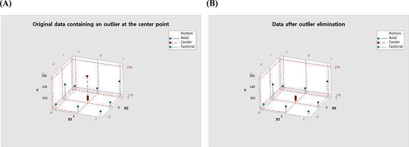
In Table 1B, runs with standard order numbers 9 through 13 are the center runs, and the responses from these runs are 260.5, 186.433, 181.933, 175.633, and 180.333. Among these values, obviously 260.5 is an outlier, and if the reason for this observation is not an error in measuring or typing, this value should be eliminated. 3D scatterplots in Fig. 1, which graphically compares the data containing an outlier and the data without an outlier, say that at the center point, 260.5 is an extreme outlier.

Now, let us see what happens if statistical models are fitted to the dataset that contains this extreme outlier.
First, let us fit to the data the second-order polynomial regression model containing 2 linear, 2 quadratic, and 1 interaction terms by using the RSREG procedure of SAS/STAT. Results of analysis of variance for this model are shown in Table 2A.
| A. Analysis of variance for the 2nd-order model on the original data in Table 1A | |||||
|---|---|---|---|---|---|
| Model terms: X1, X2; X12, X22; X1X2 | |||||
| Source | Degrees of freedom | Sum of squares | Mean square | F-value | p-value |
| Model | 5 | 988.452 | 197.690 | 0.21 | 0.9460 |
| Error | 7 | 6,489.923 | 927.132 | ||
| Total | 12 | 7,478.375 | |||
| Root MSE=30.4488 | Coefficient of variation=15.80% | r2=0.1322 | |||
| B. Analysis of variance for the one-way ANOVA model on the original data in Table 1A | |||||
|---|---|---|---|---|---|
| Model terms: Design points 1, 2, 3, 4, 5, 6, 7, 8, and 9 | |||||
| Source | Degrees of freedom | Sum of squares | Mean square | F-value | p-value |
| Model | 8 | 2,373.117 | 296.640 | 0.23 | 0.9622 |
| Error | 4 | 5,105.258 | 1,276.314 | ||
| Total | 12 | 7,478.375 | |||
| Root MSE=35.7255 | Coefficient of variation=18.53% | Maximum possible r2=0.3173 | |||
| C. Analysis of variance for the 2nd-order model on the data in Table 1C | |||||
|---|---|---|---|---|---|
| Model terms: X1, X2; X12, X22; X1X2 | |||||
| Source | Degrees of freedom | Sum of squares | Mean square | F-value | p-value |
| Model | 5 | 991.581 | 198.316 | 0.78 | 0.5962 |
| Error | 6 | 1,517.422 | 252.904 | ||
| Total | 11 | 2,509.003 | |||
| Root MSE=15.9029 | Coefficient of variation=8.50% | r2=0.3952 | |||
| D. Analysis of variance for the one-way ANOVA model on the data in Table 1C | |||||
|---|---|---|---|---|---|
| Model terms: Design points 1, 2, 3, 4, 5, 6, 7, 8, and 9 | |||||
| Source | Degrees of freedom | Sum of squares | Mean square | F-value | p-value |
| Model | 8 | 2,449.393 | 306.174 | 15.41 | 0.0230 |
| Error | 3 | 59.610 | 19.870 | ||
| Total | 11 | 2,509.003 | |||
| Root MSE=4.4576 | Coefficient of variation=2.38% | Maximum possible r2=0.9762 | |||
The model in Table 2A has a very poor fit; its model p-value=0.9460 is so large that it is close to 1, whereas the p-value of an acceptable model is no larger than 0.05, and its r2=0.1322 is so small!
Now, let us find the maximum r2 that can be obtained through the statistical modeling of this original dataset. The r2 of the one-way ANOVA (analysis of variance) model on 9 design points, which are designated in Table 1B, is such an r2. This one-way ANOVA model is the fullest model among the models that can be fitted to this dataset. Table 2B displays the results from this modeling.
The model in Table 2B has also a poor fit; its model p-value=0.9622 is so high that it is near 1, and its r2=0.3173 is still too low!
Thus, there is no way for the model displayed in Table 2A to be improved. Now, our remedy is to remove the observation with run number 2 that has the outlier 260.5 at the center point. Let us try it. Table 1C displays the dataset from which this outlier has been deleted.
Now, let us fit to the data in Table 1C the second-order polynomial regression model containing 2 linear, 2 quadratic, and 1 interaction terms by using RSREG procedure of SAS/STAT. Results of analysis of variance for this model are shown in Table 1C.
The model in Table 2C is better than that in Table 2A, but still unsatisfactory; its model p-value=0.5962 is still large, and its r2=0.3952 is still small! This implies that the second-order model is insufficient to represent this dataset. But, it may be possible for the model to be improved enough to well explain data. To check this possibility, let us also find the maximum r2 that can be obtained through the statistical modeling of this reduced dataset. The r2 of the one-way ANOVA model on 9 design points, which are designated in Table 1C, is such an r2. This one-way ANOVA model is the fullest model among the models that can be fitted to this dataset. Table 2D displays the results from this modeling.
Now, the model displayed in Table 2D is satisfactory in its ability to explain the data; its model p-value=0.0230 is lower than 0.05, meeting the criterion on the p-value for an acceptable model, and its r2=0.9762 is large enough!
This implies that the model in Table 2C can be improved by adding some proper terms to the model. Now, such an augmentation of the model to improve it in the case of a cubic central composite design, which is our case, is another topic for research. This research has been done, and a satisfactory model has been found! However, to focus on one topic at a time, the presentation of the result of this research will be given in the next article.
Conclusion
The suggestion of this research is simple: “Look at center runs before setting up the final model that explains data. If there are outliers at the center point, examine them, and they are not due to the errors in measuring or typing, just get rid of them. If the outliers are due to such errors, correct them.” This suggestion is easy to implement, and will help enhance the quality of response surface analysis in sciences including food science of animal resources.


